|
|
Backgammon AI |
Backgammon Computer Program
| |||||||||||||||||||||||||||||||||||
| Originally published in Artificial Intelligence, vol. 14 (1980), pp. 205–220. Copyright © 1980 by North-Holland Publishing Company. This research was sponsored by the Defence Advanced Research Projects Agency (DOD), ARPA Order No. 3597, monitored by the Air Force Avionics Laboratory under contract F33615-78-C-1551. |
| Abstract. On July 15, 1979, a backgammon computer program beat the World Backgammon Champion in a match to 7 points. This is the first time a world champion in a recognized intellectual activity has been defeated by a man-made entity. This paper examines the scientific issues involved in constructing the program, an analysis of its performance, and the scientific significance of the win. We also present our SNAC method of constructing evaluation functions. |
|
Contents |
Why should backgammon be an object of interest to science? Backgammon (Magriel 1976) is a game of skill and chance. The chance element is introduced by the throw of dice at each player’s turn. The skill comes in selecting the best move associated with the actual dice throw, and in making correct decisions in connection with doubling. Doubling is an action that a player can take that doubles the stakes under which the game is being played. The player being doubled has the choice of giving up the game at the current stake, or continuing the game at doubled stakes with the proviso that only he can make the next double. There is considerable skill involved in making, accepting, or rejecting such doubles.
There is skill involved in selecting the best move too. At a gross level of understanding, the best move is the one that does the most to further one’s own objectives and impede the opponent’s. Furthering one’s own objectives can take the form of actually achieving a known good that is relatively permanent, or creating conditions for the likely achieving of such good by creating opportunities for favorable dice rolls in the near future. Impeding the opponent involves making it as unlikely as possible for him to roll combinations that will help him in the near future.
The domain of backgammon comprises some 1020 positions. Its complexity approximates that of bridge or checkers, both of which can be played as an avocation or very seriously. The playing of excellent backgammon requires the application of considerable amounts of knowledge and intelligence.
Backgammon probably cannot be played by using the chief crutch of most game-playing programs—the look-ahead tree search. This is because the throw of a pair of dice can produce 21 different results, and each such throw can be played about 20 different ways in the average position. Thus a look-ahead would have to acquiesce to a branching factor of about 400 for each ply of look-ahead, an exponential growth rate that could not be tolerated very long. Thus a computer backgammon program would appear to require evaluation much more than search, very much as humans play the game.
If one uses a linear polynomial evaluation function (one that has a constant coefficient and a single variable per term) in a large domain such as chess, one soon finds out that the function is not sensitive enough. There are features that are important in the opening that are meaningless in the endgame. A linear polynomial will not be sensitive to such problems. The best it can do is to indicate the average value that should be associated with a feature. Experience indicates that this is not sufficient for expert level performance. Samuel’s (Samuel 1959) research first indicated this. Further, Samuel found (Samuel 1967) that when he used nonlinear terms (where two or more features were related in the same term) his program’s performance did not improve. This seemed a puzzling result.
An obvious solution to the deficiencies of the linear polynomial is to break the game up into phases. However, we had previously found (Berliner 1970) that having game phases for chess also was fraught with difficulties, a condition that was found to exist in backgammon too (Berliner 1977). As an outstanding example of such a difficulty, consider the fact that sound advice in chess to keep one’s King safely in a corner during the middle game, and use it aggressively during the endgame. The fact that the middle game metamorphoses into an endgame creates the difficulty. In such a scheme, there must be a criterion for deciding whether a position is a middle game or an endgame. If a program is faced with an unfavorable endgame situation and a favorable middle game situation, it will go to great extremes to avoid going into an endgame even though the current position is really very close to an endgame, and the endgame is basically unavoidable anyway.
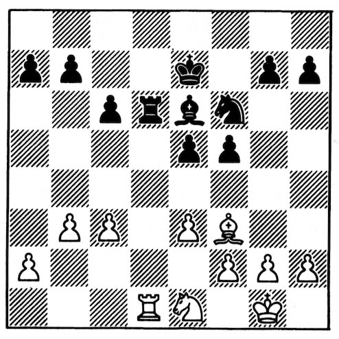
Figure 1. White to play.
Consider Figure 1. Suppose our evaluation function is designed so that with the material present in the figure it is treated as a middle game, but if one more piece were traded then it would be an endgame. Treated as a middle game, White’s King would be considered safe and Black’s exposed. In the endgame, White’s King would be considered decentralized, while Black’s is centralized. Thus, White would very likely move his Rook in order to avoid the swap and thus consider the position as a middle game with some favorable aspects, rather than an endgame with many unfavorable aspects. Yet this is a very bad action by White as it only increases Black’s advantage by making his Rook even stronger, while not avoiding the changing of the character of the position into an endgame.
This behavior is similar to that produced by the horizon effect (Berliner 1973), which causes a program to believe it has remedied an irremediable problem due to idiosyncracies in the way it conducts its search.
Expert human beings do not have problems such as those above. This convinced me that there was a great deal left to be learned about the structure of evaluation functions. However, investigating evaluation functions in the context of chess creates special problems. In chess, searching interacts with evaluation. Certain positions are considered too volatile to evaluate, so a quiescence search is performed until a set of stable positions is reached. Also, searching for a particular reason (or just brute force searching) will sometimes discover the achievement of some goal that was not at all contemplated when the search was initiated. In such situations move selection is a function not only of knowledge but also of a discovery search. In order to avoid this type of contaminant in investigating evaluation, it was necessary to find a domain that was reasonably complex and where searching had no utility. That is, it should be possible to make decisions based solely on static evaluation, and have evaluation functions to do this. Backgammon appeared to have the desired properties, and in 1974 we began developing a program to play backgammon. The next five sections present the outcome of the research into the structure of evaluation polynomials. They are taken substantively from (Berliner 1979).
When it is not reasonable to expect the solving process to search toward a terminal state, we must have recourse to knowledge to lead the way to a goal. The knowledge is in the form of “properties” or “features” that can be used to describe any state of the domain. Each such feature can take on a range of values and thus defines a dimension in a hyperspace of features. A polynomial that is the sum of various functions on these features is used to assign value to nodes and thus locate them in the hyperspace. These values are then used to order the nodes with respect to their goodness (closeness to goals of the domain).
The features that are used can represent many facets of the subject domain. Usually, things that are part of the minimal description of a state are also good features. An example from chess might be the location of the King. Other features can be more complex, or patternlike and require the operation upon several primitive features to produce a new feature. This process can be iterated. For instance, to create a feature representing blockading in backgammon it is necessary to first know the location of all (blockading) points on the board that have two or more men of a particular side on it (primitive). Then it is necessary to scan the board to find the location from which it will be hardest for an opposing man to pass through the set of blockading points, and to measure this difficulty. This is definitely not a primitive notion. In fact, it requires a good deal of experimentation in order to determine a function on the set of points that produces a good mapping into the human notion of blockading. The result will be a new feature, and its values will be used in measuring something about the value of a backgammon position.
The selected features are then combined in a polynomial function that is capable of ordering the states of the domain. The chief problem is how to do this so that the ordering is effective. Below, we present the details of our SNAC method (for Smoothness, Nonlinearity, and Application Coefficients) which appears to have remedied all methodological problems in evaluation noted above.
However, a linear function is very well behaved. In contrast, multiplying two variables, each of which could have a range of 0:50, produces a resulting range of 0:2500. The contribution of such a term to the evaluation could vary widely, causing stability problems for the value of the polynomial. Nor would normalizing the result be very satisfactory, since that would essentially suppress any variation at the lower end of the scale.
Another type of problem with nonlinear functions is the suicide construction, which we examine below. Say we have some advice to the system in the form of S = I × D, where S is suffering, I is the intensity of pain, and D is the duration of pain. The object is to minimize the value of S (as there will be a minus sign in front of this term in the polynomial). This seems to be a well-formed piece of advice. People, in general, understand that the idea is to reduce both I and D. However, a program that is allowed to manipulate D, when faced with excruciating pain that is difficult to remove, may well recommend suicide, i.e., drive D to 0 at any cost. This usually does not qualify as a solution. However, such advice can be forthcoming even when some other term of the polynomial places a large premium on staying alive. We therefore term a relation, where there exists the potential to manipulate one of the variables in a generally undesirable direction, a suicide construction.
Nonlinearity is desirable because of the increased sensitivity it provides, while care must be taken to control volatility and avoid the suicide construction.
Considerations such as the above have been studied in numerical analysis. In fact, the above may seem so obvious that the reader would feel that no one could possibly overlook such a thing. However, this is far from the case. There is very little published on the structure of evaluation polynomials that are used in game playing programs. One exception is the work of Samuel (Samuel 1959, 1967). Samuel investigates how to achieve nonlinearity without creating an unstable function. His solution, in both cited works is to map a variable with a large range onto a small range. In the earlier work, he creates “binary connective terms” which are a reduction to a binary value of a range that was large to start. Clearly, this will cause the blemish effect in the vicinity where the value of the variable changes from 0 to 1. In the later work, large ranges are reduced to ranges of from 3 to 7 in order to fit more easily into a “signature table” of limited size. Again, the blemish effect will occur near the locations where the value changes occur. We conjecture that the reason that Samuel’s program did not perform better after learning nonlinear functions is that the blemish effect caused it to commit serious errors occasionally. Consider the curves in Figure 2, which depict the situation.
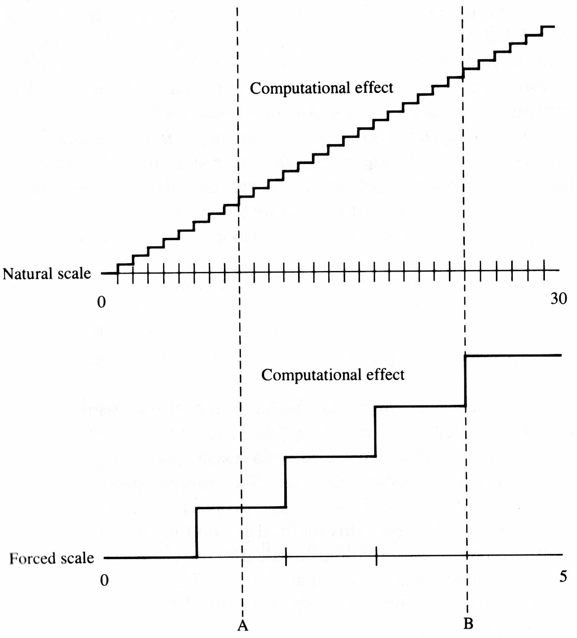
Figure 2
If the value (along the x-coordinate) of the feature is near the vertical line labeled A, then in the upper curve small variations along the x-coordinate will only produce small variations in the y-coordinate, while in the lower curve they produce no variation at all. However, near the vertical line labeled B, the situation on the lower curve is quite different. Here small variations in the x-coordinate can produce a marked change in the y-coordinate. If the value on either side of the sudden change point can be interpreted as being favorable to the program, it will go to great lengths to select an alternative for which the value will be on that side. We now are able to observe the blemish effect in the performance of older versions of our backgammon program. Thus, one suspects that this difficulty is of very widespread occurrence.
Whenever the coefficient of a nonsmooth term is under the control of the program, the blemish effect can occur. That is what causes the program to make the wrong move in Figure 1. A correct definition of endgame as a smooth function from early middle game to late endgame would appear to avoid this type of problem completely. In this way, the degree of endgameness increases with each swap of material. It is interesting to note that smoothness, thus invoked between known data points creates a transition that is not clearly derivable from the data. Yet, this appears requisite for proficient performance. Further, our studies indicate that the shape of the transition curve does not appear to matter very much.
There are two ways of achieving this additional context: (1) by fixing the value of the variable to be that in the original problem situation (frozen variable), i.e., not recomputing it for each new node; and (2) by choosing variables that vary slowly (application coefficients). We have used both methods successfully.
Using the value of a frozen variable gives the problem solving process a global outlook, where all terms using this variable are viewed as they would have been in the original situation. This has the advantage of not letting small variations create too much of an effect, and suppressing volatility for large variations. It has the disadvantage of making the process insensitive to certain kinds of changes. This method is good for functions that require some discrimination to determine the degree to which they apply, but are not required to discriminate minimal changes. This method has been used previously for efficiency reasons, when the cost of recomputing the variable at each new node is high.
The other method is to use application coefficients. An application coefficient is a variable that tends to vary slowly with operator applications (moves) due to the nature of the domain. Thus for a set of nodes that are a few operator applications apart, the value of the variable will tend to be relatively constrained. This results in a coefficient that will provide sensitivity without volatility. We give examples of typical application coefficients below.
Our typical evaluation polynomial is of the form V = A1F1 + A2F2 + . . . + AnFn, where the Ai’s are application coefficients or frozen variables, and the Fi’s are functions of features of the domain. We have found that, while there are usually many dozens of useful Fi’s in a domain, on the order of six or fewer applications coefficients appear to emerge. These are strongly related to ideas such as game phase, ease of winning, readiness for attack, etc.
In chess, typical application coefficients are:
Similar application coefficients exist in backgammon. Such application coefficients provide a program with context for making decisions. Thus a program that understands the stage of the game in chess, as a function of amount of material on the board, will allow its King to gradually achieve a more central position as the amount of material diminishes. Further, the suicide construction can be avoided by using a frozen variable in place of one that can be varied adversely. In the example quoted earlier, the duration of life of the subject becomes frozen, and that value must be used in all functions that could otherwise be subject to the suicide construction.
The results of these tests are shown in Table 1. The best program we had before using the SNAC method was called BKG 8.0. This program was the result of about 30 man-months of effort. BKG 9.7 was the result of about 8 additional man-months of work, and BKG 9.8 another additional 5 man-months beyond that.
|
Table 1. Test results of backgammon program performance.
|
||
|
BKG 8.0, 1977 (without SNAC) |
BKG 9.5–9.8 (with SNAC) |
|
| Problem set from book | 45% | 66% |
| Versus best commercial microprocessor | 56% | 78% |
| Matches against humans | 0–2 | 3–1 |
| Versus each other | 37.9% | 62.1% |
In tests on the problem book, BKG 8.0 achieved a score of 45% based on 74 problems that it could attempt. This was a peak performance for this version in the sense that the problems had been used to set certain parameters in the program, thus making it unlikely that small changes in the program would further improve performance on the problem set. Without any pretesting, BKG 9.7 achieved 66% on the full set of 77 problems in the same book, and it is highly probable that several additional percentage points of performance could have been gained by small adjustments in the program. However, we have in the last year discontinued the practice of doing this type of tuning as it has been found that many of the problems in books are too contrived (they come up very rarely), and even then answers given by the book are quite often wrong.
Against the best commercially available backgammon microprocessor, BKG 8.0 achieved 56% of the points, while BKG 9.5 (considerably inferior to BKG 9.7) scored 78% of the points in a set of 100 games. BKG 9.7–8 are now much too good to make testing against the microprocessor an interesting task. Our latest tests pitted BKG 8.0 vs. BKG 9.7–8, with BKG 9.7–8 scoring 61.1% of the points.
BKG 8.0 played in the Carnegie-Mellon University backgammon championships in the spring of 1978 and lost its first two matches thus being eliminated. In May 1979, BKG 9.7 played in a tournament of intermediate players in Portola Valley, California and won its first two matches before losing to the ultimate winner of the tourney in the third round. The competition in the California tournament was somewhat better than that in the earlier tourney. Now there is the additional win of the match vs. World Champion Villa. Finally, in October 1979, BKG 9.8 beat Barbara Glazer, winner of the strong Chicago Invitational tournament, in a single exhibition game. This is the complete performance record of all versions of our program in organized competition.
The reason for all the above accomplishments is the excellent context sensitivity, and the lack of continuity problems that the SNAC method has brought to bear on the backgammon playing ability of the program. Although versions of BKG beyond 8.0 do have approximately 15–20% more information about backgammon in them, this in no way could account for the difference. In books, problems usually come in pairs where different plays are correct in somewhat similar situations. For a program to solve both problems of such a pair correctly, it must have enough context sensitivity. If this is obtained by having a boundary between the two applicable cases then the boundary must be correct not only for this pair of cases but for all potential pairs of this type. That is frequently asking too much from such a knowledge structure. The smooth phasing over between opposing ideas that is typical of SNAC functions is much more likely to provide both the adequate context due to nonlinearity and the discrimination of those cases that are far enough apart so that they should be handled disparately.
BKG 8.0 has been available on PDP-10 machines for some time and has been regarded as a good game-playing program, and by far the best backgammon program around. Yet, as the above results indicate, the SNAC method has resulted in a rather significant improvement in the program. In evaluating the above, the reader should bear in mind that in backgammon, chance plays a significant role. In the short run, small percentage differences favoring one player are not too significant. However, in the long run a few percentage points are highly indicative of significant skill differences. A 60% edge is quite extreme.
A minimal analysis of the games from the match with Villa has been performed. There were five games in all; BKG 9.8 winning four (doubling accounted for the remainder of its 7 points) and Villa one. The analysis confirms that Villa, as expected, is certainly the better player. Although both sides made some mistakes, BKG 9.8 made two mistakes that could have hurt it very much, but didn’t due to a fortunate occurrence at the end of Game 3. Villa did not make any serious errors. BKG 9.8 made several outstanding moves (truly outstanding when one considers they were made by a machine), while Villa had little opportunity to do anything sensational because his style or the opportunities in the games did not permit this.
Villa played 80 nonforced moves during the match. In giving these games to BKG 9.8, and asking it to move in Villa’s situation, it 51 times chose the same move as he. Of the 29 times the program would have played differently, there was one occasion where it chose a clearly better move, and seven times when it chose clearly inferior alternatives. The remaining 21 differences would require a cadre of better players than myself to adjudicate their merits. It would have played one game (Game 4) exactly as Villa did.
As to the program’s own play, it made at least eight plays ranging from doubtful to obviously bad. However, only one of these bad moves was made in a situation where it could hurt. The other bad moves were bad in a technical sense only; there was a clearly better move, but its betterness would not cause a large difference in the probable outcome of the game. Most of the remaining moves were good, although I do not feel completely qualified to comment on their quality.
BKG 9.8 made a double that ended Game 2, and was considered excellent by watching experts, and was certainly quite remarkable for a machine. The double came in a volatile situation where the game could easily have swung badly against Villa. He declined the double, though the consensus was that he should have accepted. BKG 9.8 made a serious error in accepting a double in Game 3, where expert consensus said it should have declined.
However, the most revealing comments about its play can be summarized as follows: Spectators came to laugh at what was expected to be a mediocre attempt to capture the wisdom of backgammon. Instead they were treated to steady play, wherein mistakes were so few and subtle that only the very best players could discern them. In between, the program showed a great deal of imagination in making correct moves that sometimes even the experts did not anticipate.
This event was not a match for the World Championship. My program did defeat the current World Champion, but it was an exhibition match not involving the title. Further, a match to 7 points is not considered very conclusive in backgammon. A good intermediate player would probably have a 1/3 chance of winning such a match against a world-class player, whereas in a match to 25 points his chances would be considerably diminished. At the time of the match the bookmakers in Monte Carlo were quoting odds of 3 to 2 if you wanted to bet on the machine, and 1 to 2 if you wanted to bet on Villa. Thus the bookmakers apparently thought the program to be very slightly better than a good intermediate player. It would be much more useful in evaluating BKG 9.8’s strength to have played a longer series or a number of shorter series, but that will have to wait for some future time.
Further, the conditions of play may have worked somewhat against Villa taking the program seriously at first. It had been arranged that BKG 9.8 would be encased inside a backgammon playing robot as a special feature of the event. Backgammon players in general were aware of the playing capability of microprocessors already on the market, and quite logically assumed that this one would not be much better. Journalists who competed against the program in the week prior to the match found out differently, as they lost approximately 80% of their contests with BKG 9.8. However, this was not general knowledge and would probably have been discounted by the experts anyway. Further, the robot gave a semicomic impression during the event, rolling around controlled by a remote radio link and occasionally speaking and bumping into things. An uninformed person would surely have thought it was there strictly for the entertainment of the participants. However, there was $5,000 at stake, and even a World Champion should be serious for that much money. It should also be pointed out that BKG 9.8 had somewhat the better of the dice rolling. However, its dice were being rolled by a human assistant, not by itself.
On the positive side, the program greatly impressed the spectators, who had thought of the match as largely a publicity stunt, but now came to realize that the program played very well indeed. As related above, the program made a number of outstanding imaginative plays, while never going off the deep end in its use of imagination. This is highly significant, as one of the standard criticisms of programs is that they have no imagination and no understanding of strategic concepts.
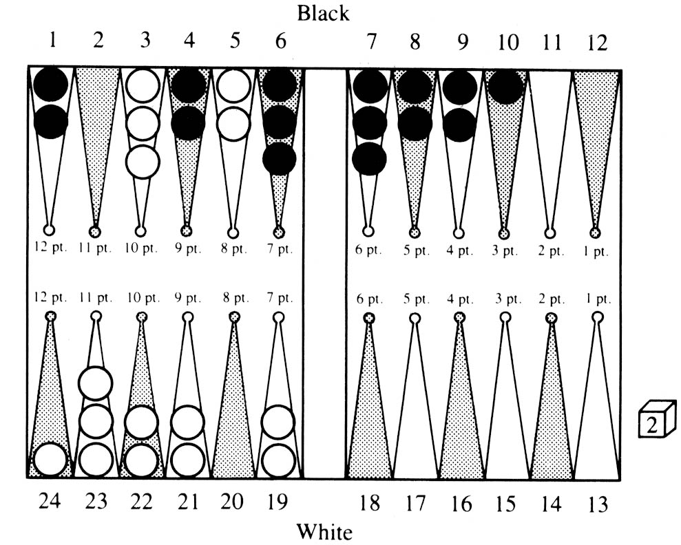
Figure 3
In Figure 3, which portrays a situation from Game 5, BKG 9.8 shows its excellent grasp of strategy. BKG 9.8 is playing White and has been playing a backgame, predicated on holding the 3 and 5 points against Black’s attempts to bring his men home. White now rolled an unfortunate double 2. Many players would be tempted to play 3/5, 19/23, 19/21 to hold their backgame position. However, BKG 9.8 realized, as would professional players, that without a good home board the backgame is useless and only risks getting gammoned. Therefore, BKG 9.8 played 3/5(3), 22/24, giving up its backgame and getting ready to run to limit its losses to a single game. Its understanding in this case was widely approved of by the professional players present.
A win in a game of skill and chance is never as convincing as a win in a game of pure skill. However, at the moment one cannot find programs that are capable of competing against top players in activities such as bridge and poker, both games of skill and chance. Measurement of skill in such games is much more difficult that it is in games of pure skill. However, such skill most definitely exists, and in order to compete on near equal terms with a world-class player, one must have a degree of skill that is comparable. This has clearly not been achieved in any of the other games of skill and chance.
Actually, the developmental aspects of the program have had a very interesting effect on my own play. When I began this program, I was little more than a beginner at backgammon. In the process of formulating issues, my own play improved considerably. Since the program can do simulations of an input position by playing it out a large number of times, it has been possible to use it as a scientific tool, both to generate new data for the program itself, and to increase my understanding of backgammon. Although I believe I am still a slightly better player than the program, it is clear that this will not be the case very much longer. The program, as one would expect, is quite inexorable in situations that it understands well. When playing against it, I sometimes ask it to suggest my best move (a playing feature of the program). On such occasions I have a correct response in mind. About 5% or more of the time the program now suggests a better move than the one I had in mind, something that I consider an omen of things to come.
Here the comparison with chess programs is apt. The top chess programs are highly dependent on search speed for their success, while my program moves almost instantaneously. This is because it does essentially no searching, instead doing a lengthy computation in evaluating each alternative in the current situation. Recently, advances in computer chess have been closely related to computing speed, although no doubt some advances would be possible with better evaluation. However, since literally hundreds of thousands of terminal nodes are evaluated in a chess search, efficiency of evaluation is a prime consideration because each additional instruction dedicated to evaluation will be executed those hundreds of thousands of times, creating significant speed decrements in the program. In backgammon, with the program doing no searching the situation is very different. What is required is to bridge the knowledge gap between where the program is now and what is presently known about backgammon. Since functions already in the program are performing excellently, it seems likely that it will be possible to keep adding new knowledge in the same manner as has been done up to now. Each such addition should do something to close the knowledge gap. Further, there is a great deal of disagreement about correct moves between top backgammon players. The advent of computer simulations into backgammon has made it possible to get relatively exact values for situations that could hardly have been appraised analytically. Overall it is clear that backgammon theory is still at an early stage of evolution, compared to games such as chess, checkers, and Go, where large bodies of undisputed theory exist. If it is possible to construct strong models of various facets of backgammon play, then it would seem likely that a program would establish new theories and standards of play on its way to becoming a true World Champion.
The recent improvement of the program is due to the SNAC method that made it possible to:
The program at present is probably as capable in its domain as any heuristic program, but not significantly better. However, since its performance is predicated on knowledge rather than search (as is the performance of most chess programs), we expect to continue to produce significant increments in its performance by merely adding new knowledge, a process that under the SNAC method has worked extremely well thus far.
We feel that there are some important lessons to be learned from this work. When chess clouded the evaluation issues that had to be investigated, a domain that did not have these problems was chosen and this allowed substantial progress to be made. Further, the fact that backgammon programs can be tested (as can all game-playing programs) in organized competition allows the reliable detection of quantitative differences in skill. This forces a program developer to face up to the issues of how good his program really is, and what can be done about it. It is this facet that, in my opinion, has been most prominently responsible for the tremendous upsurge in strength of the chess playing programs in the last decade. In the absence of such opportunities for definitive testing, the world must rely on expert testimony to evaluate AI systems. This is clearly less desirable.
![]()
|
| Articles by Hans Berliner |
|
| Articles on programming backgammon |
|
| Match transcript |
|
Return to: Backgammon Galore |
|