|
|
Backgammon AI |
BKG, a Program That Plays Backgammon
| |||||||||||||||||||||||||||||||||||||||||||||||||||||||||||||||||||||||||||||||||||||||||||||||||||||||||||||||||||||||||||||||||||||||||||||||||||||||||||||||||||||||||||||
| Originally published in July 1977 by the Computer Science Department, Carnegie-Mellon University, Pittsburgh, PA 15213. This work was supported by the Advanced Research Projects Agency of the Office of the Secretary of Defense (Contract F44620-73-C-0074) and is monitored by the Air Force Office of Scientific Research. |
|
Abstract. This paper is both a description of an existing backgammon program and a theoretical discussion of some important issues in evaluation. The program plays a generally competent game at an intermediate level of skill. It correctly solves a high percentage of intermediate level problems in books. Although it only doubles and accepts doubles during the running game, it does several nontrivial things perfectly. In discussing the structure of evaluation, we consider partitioning all game states into mutually exclusive state-classes. These state-classes are very useful in a knowledge-based system, as they allow relatively easy assimilation of new knowledge. They also permit the building of opponent models based upon what evidence shows the opponent knows in each state-class. |
|
Contents |
The thing that makes backgammon an interesting object of study of AI is that in any given position (of which are 1020 (Levner 1976)), there are 21 possible combinations that the throw of two dice can produce. Each of these can be played legally in the average board position about 40 different ways. Thus if one were to investigate a backgammon position by tree searching it would be necessary to deal with a branching factor of more than 800 (!!) at every node. Clearly, this is completely impractical. Therefore backgammon must be approached with evaluation and knowledge in mind. Position P1 will have to be preferred over position P2 because it has features that more endear it to the player who can produce it than the features that obtain in P2.
In a game such as chess, it has been customary to search very large trees of 5000 to 2 million terminal nodes. In such a paradigm, the execution of a terminal evaluation function requires a certain amount of time, which must then be multiplied by the expected number of terminal nodes in the search. Thus designers of chess programs are very circumspect in creating evaluation functions which require lengthy execution times. For this reason certain features that are not trivial to compute are usually left out, so that the program may operate faster and search more. Since there can be little or no searching in a practical backgammon program, these contingencies will not apply. On the contrary, it is desirable to apply all possible knowledge to successor positions of the root node, in an attempt to find the best next move. Further, the fact that modern backgammon involves doubling and accepting doubles places an even greater emphasis on the use of knowledge for knowing when to double and when to accept doubles. It is the encoding of knowledge and the subsequent selection effectiveness of the evaluation function that is of interest. This subject is treated in depth in Section IV and V. However, before going to that part of our research, we describe certain peripheral artifacts that are important for understanding the whole project.
BKG operates, similarly to many game playing programs, by executing a minor cycle which makes moves within a major one which plays games. When BKG is running interactively, it displays appropriate outputs and prompts at each step of the cycles.
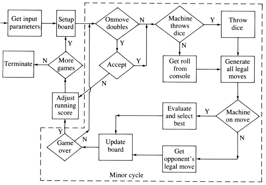
Figure 1
The minor cycle (see Figure 1) operates as follows: First, BKG checks to see if the side whose turn it now is wishes to double (checking first that it would be legal for that side to do so). If a double is made, BKG asks if the double is accepted. If so, BKG adjusts the position and denomination of the doubling cube and proceeds. If not, the game is over and BKG exits to the major cycle. Next BKG checks to see if it is to throw dice or receive a roll from the console. BKG uses a random number generator to throw dice. It then generates a list of all possible legal moves for the given roll. It it is the program’s turn to play, it serves these potential moves up, one at a time, to the evaluation procedure. It then selects the best. If it is is not the machine’s turn to play it waits to receive a move from its environment. It then checks the legal move list to see if this move is on the list. If not, it requests a legal move. If the received move is legal, BKG puts it into canonical form. It then executes the legal move by updating the board configuration. If the conditions for one side winning have been met, it exits to the major cycle.
The major cycle is activated whenever a new game is about to begin. If a game is just over, BKG adjusts the overall record of the current competition in favor of the side that just won. It then asks if another game is desired (unless it has been preset for a certain number of games and this number has not been reached as yet). If the answer is negative, the program terminates. Otherwise, it sets the board up, throws dice to see who starts, and yields control to the minor cycle.
BKG can operate in several different modes. Its usual mode is to play a human opponent interactively at a video terminal. However, it can also monitor a game between two opponents while rolling dice for both, and doing the bookkeeping for doubling and accepting decisions. It can also play itself, either while displaying all actions at the terminal, or by only reporting the results of a series of games. For this simulation mode, it is necessary to type in a starting position and the number of iterations desired. For certain types of positions that BKG can play well, this mode can be used to determine within reasonable limits of accuracy what the chances of the respective sides are.
When one or more human opponents are involved, there is the option of letting the humans throw dice for themselves and entering the roll when the program prompts for it. For ordinary purposes this is much too slow a way of playing the program. There is, however, a practical reason for this mode. In tournaments it will be necessary to actually throw dice at the table for both sides, and a method must exist for entering the rolls. It is rather interesting to note as an aside, that while we have seen quite a few illegal moves made in tournaments, this should never happen to BKG, as if a move is not on its legal move list, it would not accept the opponent playing it.
However, there are problems. First, the above procedure will generate many duplicates which we would hope to avoid or eliminate after generation. Second, and more importantly, the procedure outlined will not work for situations in which the moving side has men on the bar (and the only legal moves consist of entering men from the bar), and for those situations where all the men are in the home board (when it is legal to move men to the next point beyond the end of the board and in certain cases even beyond that). Thus on careful examination we determine that there are three distinct states that a board situation can be in:
Further, it is possible for the state to change during a single play, and the move generator must be able to come to grips with such a situation to generate all legal moves, and only legal moves. A final complication introduced by the rules of backgammon requires that if a full play cannot be made according to the roll, the player must play the largest possible part of the roll. This means that if he can play the full roll, he must do so and if he can player either die face, he must play the larger.
The move generator understands exactly what moves are legal in each of the three states. As moves are generated which could form a legal play, these are put into a tree form. When move generation has been completed, the tree is scanned and those plays that are legal by our final criterion (use maximum part of roll) are marked as legal plays.
In view of these considerations, we implemented the move generator in the following way. We have a recursive procedure which can call itself a maximum of three times (for doubles) and once for nondoubles. The procedure starts at the location of the man that is furthest away from home for the moving side. It then scans toward home, pausing each time a point is found containing one or more men of the moving side. The die faces are labeled arbitrarily FACE1 and FACE2. The move generator first determines which of the three states the board position is in. It then attempts to apply the current die face to a man on the current point. If it fails in this, it continues the scan until there are no more men or points, whereupon it backtracks. If it succeeds, it updates the board, and if there are still move die faces to apply, it calls itself. In this case, a parameter of this call is the point at which the next scan should commence. For nondoubles this is the same point where the first recursion began. However, for doubles a large saving can be realized by using the current point as argument (since all opportunities to apply the denomination of the die face earlier in the recursion must already have been tried!!). This algorithm will generate all legal moves and only legal moves. For instance, in the case of doubles, if there are more than one man on a point, when the recursive call occurs, the algorithm will attempt to apply the remaining die faces to be played to the remaining men on the point before continuing the scan. Thus, for doubles this algorithm will not generate duplicate plays, while for nondoubles it will. For this reason we use a small modification of the procedure for nondoubles, but this does not concern us here.
It is generally considered by backgammon experts that doubling is what separates the men from the boys (meaning that it is relatively easy to make the right move most of the time but hard to know when a position is good enough to double and bad enough to refuse an opponent’s double.) To implement even a mediocre doubling and accepting algorithm is an extremely difficult task. Because of this, BKG at present only permits doubling (in games in which it is playing) in situations where the two sides have disengaged so that captures are no longer possible. This limitation is being remedied in the version we are currently working on. The problem of constructing such decision algorithms are treated in later sections; here we discuss only the requirement for the program to handle doubling in game.
Since it would be rather boring to ask each human player before his roll (if he were legally entitled to double) “Do you want to double?”, we have instead created a doubling flag for each human opponent. If a human feels he may want to double on the next roll, he should enable the doubling flag before making his current move. This will result in BKG prompting him with an asterisk before the dice are rolled for him next time (and until the flag is turned off). When the prompt appears, the player may double or just continue. When the doubling flag is not set, BKG will just roll the dice without asking about doubling. This speeds up the game considerably. Of course, for itself BKG does not need such a flag as it can consider its doubling actions in a few microseconds.
When BKG has been doubled, it decides whether or not to accept using the same procedures it uses in deciding whether to double. Whenever a double has been accepted or rejected, the bookkeeping decisions that follow are rather trivial.
There are many intricacies to appraising the danger that a set of blots is in. When we first brought the program up, BKG merely noted the existence of blots. It considered all blots equally likely to be hit, and merely delivered a value that represented the total pipcount that would be lost if all blots were to be hit. This was term that the evaluation procedure attempted to minimize.
However, this measure proved very inadequate; it failed, most importantly, to consider whether any particular blot could be hit by an opposing man. Our next (very small) improvement was to determine that for a blot to be in danger at all, there would have to be an opposing man somewhere in front of it. This produced a small improvement in performance. However, it still failed to get at the degree of endangerment of any blot.
Next we noted that for a blot to be hit it must be a distance of 1, 2, 3, 4, 5, 6, 7, 8, 9, 10, 11, 12, 15, 16, 18, 20, or 24 in front of the hitter, and that for each such distance there is a hit probability corresponding to the number of possible combinations. This new fact produced a very large increment in performance, but it still left untouched several important situations. One of these is that even when a hitter is the right distance away from a hittee, it is at times necessary to have available a set of intermediate points where the hitter is to land. Second, is what is called in backgammon jargon duplication: it is impossible to apply a single die face to more than one move. Thus there is a certain safety for a pair of blots if they can be hit by different men (say) 4 pips away. The point is that if a 4 is rolled only one of the blots can be hit, but not both. Third, there was the question of more than one blot being hit with a single roll (something that is usually wise to avoid), and the question of a single blot being hit simultaneously by two men. This is known as pointing on a blot, and is also something that is wise to avoid.
As a result of these considerations, we finally implemented a very detailed hit probability procedure which we now describe. We consider any man which is not paired on its point to be a blot, unless it is on the 1 or 2 point in the opponent’s home board and the opponent has not yet made more than two points in his home board. We consider any man to be a hitter unless it is part of a pair (and only a pair) in its home board. The reason for the latter is that moving one of such a pair would expose the other to the hittee coming in on the next play, and thus would not really constitute a threat.
We note that there are 40 different ways in which an arbitrary hitter can hit a hittee. To illustrate this consider that there are three different ways in which a hitter three pips away from a hittee can hit it: by a 3, a 2-1, or using 3 parts of a 1-1. This information is encoded in a table of masks which specify which intermediate points must be free, or that only one of a set of two points need be free.
Our procedure scans the board, starting with the most advanced blot of the moving side, and determines if it is in range of any hitters. If so, then for every hitter it determines all combinations that could be used to hit this blot. It then checks whether the intermediate landing point conditions are satisfied. If so, it enters the location of the hitter in the word corresponding to this combination in the 40-word vector of bit-vectors Ahit. At the end of this first pass, the factor Ahit contains all the locations of potential hitters, the combination used for the hit, and the location (implicitly) of the hittee.
Next the procedure determines whether the side next-to-move as 0, 1, or more than 1 men on the bar. There is a separate section of code for each of these situations. Basically, the procedure examines each word of Ahit to see if this combination can be used to hit a man. It starts with the combinations that use only one die face and then goes to the more involved combinations. Each time it finds such a combination it checks to see if the die faces needed for this combination have not been used yet. If so, it marks the faces as used, updates the information on hitting (always assuming that the most advanced blot will be hit if there is a choice), and continues.
If it finds that a combination using only one die face can be used to hit more than one blot, it knows that there exists a combination (the double with that die face) that can be used to hit two blots. If it finds that blots can be hit with more than one single face combination, this means either that a blot can be pointed on or that two blots can be hit with a certain throw. Whenever a blot can be hit by a combination involving two die faces, it checks whether a blot exists on either intermediate point. If so, this combination would hit two blots. In all cases, the values are multiplied by the unused number of ways that this combination can be rolled. At the end of this computation the following values are available:
These data are very adequate to the task at hand. For instance, in situations near the end of the game where one side must break up its safe position and run across no-man’s-land exposing some blots, BKG does a remarkable job of distributing blots so as to minimize the chance of any being hit. This can be quite difficult even for a master player at times, but this is one of the about three or four areas of backgammon play where BKG plays perfectly.
However, there are still some inadequacies to the current approach. The principal one is that the hit probability calculation assumes that it would be desirable to hit any exposed blot. This is usually valid but not always. For instance, the man that would be the hitter might be part of some important blockading or defensive structure and would therefore not want to give that up in order to hit a blot. Also there is the possibility that if the blot were hit it would in turn leave a blot for the opponent. Under certain circumstances (of which we already indicated one earlier) the disadvantages of leaving a blot in the process of hitting a man outweigh the advantages of making such a hit. We have in mind to improve the calculation to report which men are the hitters and name points on which opponent’s blots would be left after hitting a blot. However, the program does not seem to be as limited by the lack of this information as by some other things, so this improvement will be postponed until such a time as it seems necessary. We are also aware of the ad hoc nature of defining what is a blot and what is a hitter, and will at some future time make these definitions more sensitive to the overall board situation. However, as of this writing the hit probability computation is by far the most sophisticated thing in BKG, encompassing some seven pages of code.
Initially, we counted the maximum number of contiguous blockading points and squared this number to give greater weight to longer blockades. However, this method overlooks the fact that a blockade of six-in-a-row cannot be spanned, the fact that seven-in-a-row is not better than six-in-a-row, the fact that blockading points do not always have to be contiguous to be effective, and the fact that blockading strength is affected by the distance that a potential blockade runner is away from the blockade. To overcome these objections we developed a table of potential blockades.
We note that since there are only 15 men on a side, it is impossible to have more than seven blockading points. We then computed all combinations of zero to seven blockading points at a distance of 1 to 12 spaces in front of a man. For each configuration we computed the number of rolls that could legally be played by the blockade runner. This is the best measure of the strength of a blockade that we have found. Since a byte of 12 bits uniquely identifies any blocking configuration, and since the number of rolls that can result in getting past the blockade must be between 0 and 36, we constructed a table with bytes of six 6 bits accessed by a 12-bit code describing the blockading configuration. This method results in quick lookup of the essential data. We keep track of:
It has been found that this information satisfies our needs at the moment.
At the end of any potential play, BKG evaluates the placement of all men not yet in the home board. For each such man, BKG computes the number of board-crossings the man still has to make to get into the home board, and where the man is placed in its current board. In backgammon terminology a board is a sequence of six points (of which there are four, the two home boards and the two outer boards). In general, for the same number of total pips remaining, it is most desirable to have the fewest men left, and have them placed as far back as possible in the board they currently occupy. This allows the most efficient utilization of the most throws. Thus BKG will multiply (3 − number of board crossings) by the depth of man in his board. This function seems to produce the desired effect, because it gives the greatest weight to the location of men closest to entering the home board. If the program’s side is in danger of gammon, BKG will try to maximize potential rolls of doubles. Thus it will place men so that they can be brought home and one borne off most easily in the event of double 6, 5, 4, 3, or 2.
BKG makes and accepts doubles only during the running game. Until the position is advanced enough so that bearoff tables that give the expected number of rolls to get all men off can be referenced, it uses an algorithm developed by Emmet Keeler (Keeler et al. 1975) of the RAND Corp. This algorithm uses an adjusted pipcount which adds 4/3 pips for every man on the 1 point, 2/3 pips for every man on the 2 point, and 1/3 pip for every man on the 3 point. If one side has borne off fewer men than the other, the (Acount) of that side is increased by 2 pips for every extra man. Finally, it checks the number of gaps (points unoccupied by own men) in the home board of each side and subtracts the difference from the side having the fewest gaps. This is the adjusted pipcount (Acount) used in the following computation.
BKG will double if the cube is in the center if its opponent’s Acount is 10% minus 2 pips greater than its own. It will double when it owns the cube if its opponent’s Acount is 10% minus 1 pip greater than its own. It will accept doubles when it is not more than 10% plus 2 pips behind. This algorithm performs in a basically satisfactory way.
The tables cover all situations for up to and including eight men in the home board, and up to and including 25 pips worth of men in the home board. The latter value assures that the tables can handle situations where, for instance, one side has all his men on the 1 and 2 points, but at least five on the 1 point.
The use of the tables in move selection is simple. BKG moves to the position with the lowest ENR. There is one exception to this case; that is when it is far behind or far enough ahead to have a chance of winning a gammmon. In the former case, it moves to the position which has the greatest probability of bearing all men off in the number of rolls that are expected for the opponent to get off. Here the values of probabilities of getting off in N rolls are very useful. When it is far ahead it moves to the position which gives it the greatest chance of bearing all men off in the number of rolls it expects to have before the opponent gets his first man off. It does this by giving additional weight in the computation to the probability of getting off in 1, . . ., n rolls, where n is the number of rolls it expects to have before the opponent meets his objective.
For doubling and accepting doubles the situation is more intricate. Whenever BKG can legally double during this phase, or when it has been doubled, it executes a win probability calculation. If the bear-off position of either side is not in the bear-off probability table, then it uses the Keeler method described above. In that case, the ENR is computed to be the larger of the Pipcount/7 and the (number of men left + 1)/2. This will usually overestimate the real ENR somewhat. If the ENR’s for both sides are in the table then BKG can calculate the exact probability of the side on move winning by iteratively calculating over N the following equations:
| W ← W + (1.0 − W − V) × AWPRB(N) V ← V + (1.0 − W − V) × AVPRB(N) |
until W + V = 1.0. Here, W is probability of Onmove winning, and V is probability of Notonmove winning. The AWPRB(N) are computed from the bear-off probability tables by the following equation:
| AWPRB(N) = WPRB(N)/(1.0 − PRBZ) |
| where PRBZ = | N − 1 Σ i = 1 |
WPRB(i). |
If the moving side has a 65% chance of winning, BKG will always double. If the moving side has more than a 79% chance of winning, BKG will always resign if it is the nonmoving side. In between there are many situations in which it makes a great deal of difference how many rolls are left in the game, who has the cube (one should be more cautious in doubling when giving up the cube), and where in between 51% and 65% the win percentage is. We use a set of ad hoc tables here, and periodically adjust them when the program appears to be doubling too early or too late.
It should be noted that BKG does a vastly better job of doubling and accepting when using this algorithm than when relying on the Keeler approximation. This can be noticed, for instance, when the position is close but appears to favor one side. When the position changes so that both positions can now be looked up, BKG will frequently double, even though very little appears to have changed from the situation one roll ago for both sides. Upon inspecting the value of the win probability for the moving side, it is not unusual to find it between 60% and 65%, values which were not sufficient to activate Keeler’s approximation. For this reason, we are looking at more precise ways of dealing with running game doubling, with the view of being able to obtain an estimate of the win probability of the side on move, rather than the double/don’t double decision which Keeler’s algorithm estimates. To this end, we are looking at the work of Thorp (Thorp 1975), and have some ideas of our own for simple approximations which can be tested using our simulation facility.
An example of the kind of thing we are talking about is the position in Figure 2.
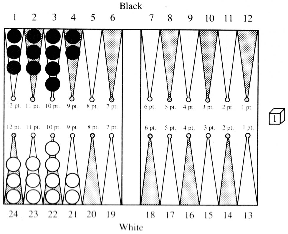
Figure 2
Here the Acount for both sides is 36. 36 × 1.1 − 2 = 38, so that Onmove cannot double. Yet Onmove has approximately a 65% chance of winning here, as evidenced by simulations. The power of the bear-off tables is very impressive. Here is another area where the program plays perfectly. To illustrate the type of thing BKG does to amaze its author, we show two examples.
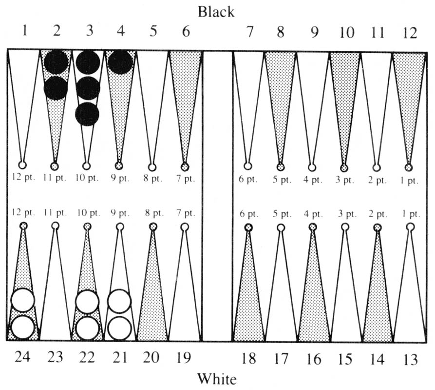
Figure 3
In the bottom part of Figure 3, White is to play a 6-2. The 6 must obviously be played from the 21 point. But what is the correct way to play the 2? Almost every human player would say 21/23. However, this is not correct; 22/24 is better. The bear-off tables report the respective ENR’s to be 2.748 and 2.739. Upon examination, it turns out that all sequences of future rolls produce the same results in the two positions except when one of the next two rolls is 1-1. If this occurred on the first roll, it would in both positions allow taking three men off. In the preferred position this would leave men on the 21 and 23 points, which allows six additional combinations of getting them both off on the next roll over the other position where the two men would both be on the 22 point. The situation is similar if the 1-1 occurs on the second roll.
The second example in the top part of Figure 3 has similar features. Here Black is to play a 6-1. The 6 must be played from the 4 point, the question is how to play the 1. Again human players would automatically play 2-1, but this is incorrect. 3-2 is better in all future sequences. Again only those sequences involving a 2-2 make a difference. This would allow getting off in two rolls unless the next roll is 2-1 in the preferred case, but would do no good in the other. The respective ENR’s are 2.794 and 2.777.
It may seem that the advantage gained by making the correct play in these cases is trivial; however, it is certainly worthwhile to improve one’s chances in the play when it can be done at no risk. For these two examples it would seem that the rule: “When there are a small odd number of men on the board, play to maximize use of doubles” would seem to be the correct way for humans to capture the knowledge that is contained in the tables.
However, as well as this does, it still leaves some things to be desired. Basically, the real issue is whether any man or men is so far behind that it we be very difficult for it to ever join the main force. Or whether any men are so far advanced that they will not play any meaningful role in the game until the bearing-off stage is reached. These two issues are probably best treated separately and we intend to do this in our next revision. It is desirable to maintain stepping stones of safe points for lagging men to join the main force, and it should be relatively simple to devise a measure of the number and nearness to each other of such stepping points as an index of the ease with which lagging men can be brought to safety. Likewise, far advanced men can be debited according to how far advanced they are beyond the last safe man of the opponent. Even with such measures available, we would still plan to retain the second moment term as a useful measure of dispersion of the total force.
To evaluate any position, we must decide which evaluation computations are applicable. The first step in this process is to decide whether it is a running game position or the forces are still engaged. We explained in Section IV how running-game evaluation is done. When the forces are still engaged the evaluation proceeds as follows:
The unit of evaluation is the heuristic point (HP). For all positions where the sides are not yet disengaged the following GENERAL evaluation is performed:
|
HP ← HP + Caploss + Ownmen(Offboard)*( if P1 = 0 then 22 else 3 ) + Mobility/5 + Getbackin(Closeboard(Justmoved), Onbar(Nexttomove)) − Piploss/Winfactor − ( if not Manhome(Mostback(Justmoved)) then Moment2 ) − 2*(Ownmen(Justmoved, 1) + Ownmen(Justmoved, 2)) − Homblots(Justmoved)2. |
The evaluation now becomes more sensitive to specific situations. First, we determine whether Acontain(Justmoved) ≤ 6 in which case Justmoved is considered near disengagement and the NEARDIS evaluation is performed:
HP ← HP + ( if Edge > 0 then Edge2 else Acontain(Nexttomove)3/300 )
− Histack(Justmoved)
+ ( if Ownmen(Mostback(Justmoved)) ≤ 2 then 10 )
(This makes it easier to break this point and move the men up)
+ ( if Manhome(Mostback(Justmoved)) then
begin
if Ownmen(Mostback(Justmoved)) mod 2 = 0 then 10;
if (Ownmen(Mostback(Justmoved))
+ Ownmen(Mostback(Justmoved) + 1)) ≥ 5 then 10;
end ).
HP ← HP − (GAP(Justmoved) + P1)
* (Contfactor + Getbackin(Closeboard(Nexttomove), 1)/4 * 6
/ Distance(Offboard, Mostback(Justmoved)).
HP ← HP + Acontain(Nexttomove)*2 − ( if Edge > 0 then Edge*3 ).
This factor is a measure of how desirable it is to be getting near disengagement, and thus encourages or discourages getting into this state.
HP ← HP + Acontain(Nexttomove)3/300.
This factor encourages maintaining the best possible actual containment because disengagement is not in the interest of Justmoved.
HP ← HP + (Expallin(Onmove) − Expallin(Justmoved))/10.
This factor encourages Justmoved to bring his men efficiently near or into the home board, while being applicable only when Justmoved’s position has no holes in it. For this section the important ideas are: If we are ahead and were near disengaged then try to bring men up with minimum danger.
HP ← HP + Slotted(Justmoved)
+ Builders(Justmoved)
− Histack(Justmoved)
+ Acontain(Nexttomove)3/300
+ Contain(Nexttomove)2/50
+ ( if Onbar(Justmoved) = 0 then
Escapes(Justmoved, Mostback(Justmoved))*2 )
− Escapes(Nexttomove, Mostback(Nexttomove))*2.
We consider if we wish to stay around in the hop of hitting a man. This is because we have some defensive potential in case we do hit the man. In that case the following defensive potential is added in:
HP ← HP + N3*Distance(Mostback(Justmoved), Mostback(Nexttomove))*2
− PRB(1)*100,
where N is the number of men that must cross, and PRB(1) is the probability of their crossing in one roll. The latter quantity is found by using the bear-off tables with the input shifted to make it appear that the edge of the board coincides with the location of Mostback(Justmoved).
HP ← HP + 150 + Acontain(Nexttomove)*3.
This encourages keeping the opponent blocked in if at all possible.
HP ← HP − (P1*(Getbackin(Closeboard(Nexttomove), 1) + Contfactor))/Winfactor
− (P2*(Getbackin(Closeboard(Nexttomove), 2) + Contfactor))/Winfactor.
HP ← HP + (Acontain(Onmove)2 − Acontain(Justmoved)2)/50.
It is noteworthy that these evaluation functions produce almost all the recommended ways of playing the opening rolls, thus obviating the need for “opening book knowledge,” and also confirming the validity of the evaluation process.
However, it is almost self-evident that one evaluation function cannot serve to order all positions. To do this, incredible complexities would have to be introduced. Consider the Slotted term. Before the opponent has built a strong defensive position, it is worthwhile to expose a man in a slotted context in order to improve one’s own position. As the opponent’s position gets better this becomes less and less worthwhile. However, in certain desperate situations, it may again be desirable to take such risks. Finally, in the running game the term has no meaning at all. Clearly, the coefficient of this term must be sensitive to a great deal of context, which in effect makes the coefficient nonlinear and the resulting evaluation function nonlinear. Rather than evaluate one gigantic nonlinear evaluation function, it seems wiser to evaluate each position in its proper context.
Thus the whole issue of state-classes and their associated evaluation functions is born. The issues associated with state-classes are these: We assume that it is possible to partition all game positions into mutually exclusive state-classes. This is not difficult and can be accomplished by merely having recognizers for a set of state-classes, invoking these recognizers in a canonical order, and putting all non-recognized positions into a grab-bag class. We further assume that within a state-class, a linear polynomial function exists which can order the members of this class according to goodness. It is apparent that this is true in the limit, when there is a state-class for each position; however, the degree to which this is possible when there are a large number of members in a given class is not clear. In practice, it is possible to get very good (if not perfect) orderings, and to split a state-class when the ordering procedure becomes too difficult.
In general, state-classes can be classified into the following categories: (1) essentially won, (2) favorable, (3) about even, (4) unfavorable, and (5) essentially lost. In all cases it is possible to further subdivide the classes into stable and unstable, where in general stability can be thought of as the variability of the end result. Thus the following ordering of these categories represents their general desirability: (1) won stable, (2) won unstable, (3) favorable stable, (4) favorable unstable, (5) even stable, and even unstable, (6) unfavorable unstable, (7) unfavorable stable, (8) lost unstable, and (9) lost stable. Frequently, in order to reach a more favorable class, it will be necessary to go first to an unstable class; i.e., take a chance. In general, the side that is closest to winning will want more stable positions and the side that is closest to losing more unstable ones.
However, this is not always the case. The side that has a slightly better position may want to introduce some instability in the hope it will result in an even more favorable position (or even won), while risking losing the advantage or possibly getting slightly the worse of it. This kind of decision is very difficult to program if all positions are evaluated only on their expectation or game-theoretic value.
Actually, notions such as progress and risk are crutches that are not needed when a universal measure of goodness such as expectation exists, as it does in backgammon. Thus we should always move to the state with the greatest expectation, and state-classes are not needed at all. However, as we pointed out earlier this is only in a system with perfect knowledge. When there is imperfect knowledge, such crutches allow for much smoother performance.
To give an example of move selection across class boundaries, consider the position of Figure 4.
Figure 4
In this case Onmove is White. The current state-class (1) is characterized by Onmove being ahead in the pipcount by 15 pips or more, having to cross exactly two more enemy points with his Mostback, and having P1 ≤ 3. We can now imagine an evaluation function for this class which would consider the position of the doubling cube, the exact difference in the pipcount, the distance between Mostback and each of the two points that must be crossed, Contain(White), the number of stepping stone points of White between the two points of Nexttomove that must be crossed, the value of Closeboard(White), and the number of pips that are available to be played as slack before any of these values are decreased. Such a function could conceivably deliver an output that would indicate the expectation of White in the particular member of the state-class. Such a function could be derived either by analytic means or by actual simulation of positions in the class to find out how each of the above variables affected the expectation of White. Further, such a function could be tuned as experience is accumulated. Let us assume that such a function exists and predicted that in the situation of Figure 4 White should win 66% of the time, win a gammon 2% of the time, lose 30% of the time and lose a gammon 2% of the time, for a net expectation for White of +0.36.
Now from this position it is possible to move to four state-classes: the present one (class I), an unstable state-class where White has two points to cross, but has a blot in danger of being hit, i.e., P1 > 3 (class II), an unstable class where White has only one more point left to cross (class IV), and a stable class where White has only one point left to cross (class III). Further, if a blot is hit in state-classes II or IV, we have another state-class (V) in which White has a man on the bar which must enter in front of Black’s blocking position. Each of these state-classes will have their own evaluation functions. Thus when deciding how to play a roll, the play yielding the best expectation will be chosen.
White’s win probability, W, in a state where he is to move is the SUM i = 1 to n (Ti*Wi) where Ti is the probability of transiting to state i on the play by playing it optimally, and Wi is the probability of winning once state i is reached. If it is Black to play, White’s win probability can be computed in a like manner.
This method can be used to decide between plays that result in differing state-classes even though one class may be unstable and the other not. Let us illustrate by an example. Assume that W = 0.92 for positions in state-class III. W for positions in state-class II is PH*W5 + (1 − PH)*W2, and W for state class IV is PH*W5 + (1 − PH)*W4. Here PH = P1/36, W2 = 0.85, and W4 = 0.92. To get W5 we must compute the probability of White escaping over the blockade on his next roll, as otherwise he will be doubled and will have to resign. If he does escape, he has about an even chance in the resulting position. These constants should make clear the computation below. It should be noted that when W for a side that is on roll and can double is ≥ 0.75 (i.e., his expectation ≥ 0.5) he can double and force his opponent’s resignation. Thus such terms should be ignored as their value drops to 0. This is true for instance of the term dealing with the situation where White is hit and contained.
We now use this method to decide how to play a difficult roll, 6-1, in Figure 4. There are basically two plays: run one man from the 12 point resulting in a position of class II, or play both men from the 18 point remaining in class I. For the first play:
| W = 20/36*0.85 + 16/36*2/36*0.5 = 0.48. |
For the second play, there are five rolls which result in transition to state class III (2-2, 3-3, 4-4, 5-5, 6-6), 2 rolls that result in a class II position (6-2), eight rolls that result in class IV positions (6-1, 6-3, 6-4, 6-5), and 21 rolls that result in remaining in state-class I. The appropriate computation is
| W | = |
5*0.92 + 8(16/36*2/36*0.5 + 20/36*0.85) + 2(23/36*2/36*0.5 + 13/36*0.75) + 21*0.55/36 |
(state-class III) (state-class II) (state-class IV, 2 blots) (state-class I, new W = 0.55) |
| = | 20.61/36 = 0.57. |
Therefore, it can be seen that it is better to make play two. It should be noted that as the probability of containing a hit man varies with Black’s defensive formation, this calculation will also vary accordingly.
The method we have described above can be used to for deciding the very important problem of when to move to a state that is in a state-class different from the one we are currently in. However, the whole method assumes that an accurate evaluation function exists for each state-class; i.e., it both orders properly and produces the correct expectation for each member of its class. This is obviously never the case.
Therefore, it is necessary to show how such a system can operate adequately and can be improved in the face of error. For each state-class there are new state-classes that can be reached in one optimal play for each side without a capture being made. We call these classes forward with respect to the original class. Likewise, there are new classes that can be reached from the current class in one optimal play by each side, when there has been at least one capture of a man. We call these classes backward with respect to the original class.
It is possible to start with a class for which we have excellent expectation data, i.e., the class of bearing-off positions that can be looked up in our tables (class B). Next, we consider all classes for which class B is forward, and improve the evaluation function for those classes, tuning the coefficients of existing terms and adding new ones as required. This will improve these evaluation functions. We also note all classes that are backward to this class, and put them on a list together with the name of the current class. We can continue this process indefinitely, but painfully, until every class has been encountered. Whenever the evaluation function of a class that is on the backward list is improved, we go back and modify all the evaluation functions of the affected classes. We can then continue our process or go back to one of the classes whose function has just been modified and start anew from there. It is clear that this is a converging procedure. It would probably be necessary to eventually automate this procedure, if for no other reason than that eventually the evaluation functions would become so good that they would do a better job of ordering members of a class than the experimenter would. Such automation, except for the introduction of new terms, has been previously done by Samuel (1959) for checkers. It would appear likely that for a game such as backgammon, it would be possible to get a selection of terms such that no new ones will ever be required. Then it will be merely a matter of tuning old evaluation functions, pulling in a new (but known) term every once in a while to see if it can improve prediction.
As data are collected and the evaluation functions improve, two things become possible. It is possible to keep track of how the prediction works out for the program’s own play, which can be used as an indicator of which functions need to be tuned next. It is also possible to keep track of individual opponent’s results and come to the conclusion that they do not appraise certain state-classes correctly, and use this information in future games.
We followed the practice in scoring the results of giving BKG part credit for answers that were not perfectly correct but showed it understood the main point of the problem, although the execution was not perfect. We also deducted part credit when it got the correct answer without understanding what the main problem was. Table 1 shows the results of the tests.
Table 1. Tests of BKG on Better Backgammon.
| Position class | Number | Right | Wrong |
Percent correct |
|
Positional Running bearoff Engaged bearoff Back game Timing Advanced defense Defense |
28 5 11 8 13 6 3 |
18.75 5 2 3.25 4 0.5 1 |
9.25 0 9 4.75 9 5.5 2 |
67 100 22 41 31 6 33 |
In evaluating these results, several things should be noted. The subject matter is relatively advanced, and would for the most part come up in only one of 20 or more games. There are usually on the order of three plausible answers to a problem. BKG is good enough in almost every case to know what these are; thus attaining a score of 33% or less could be regarded more or less as the result of chance. We can see that BKG is extremely good in running game play. Also it has a good understanding of the relative positional advantages. However, its performance in other intermediate level aspects of the game is at best mediocre. It has heuristics to help it do bearing off while still engaged, but these are for the run-of-the-mill situations, not for the more sophisticated ones in the test set. It has no specific understanding of the back game. Since the objectives in the back game are rather different than anything else in backgammon, it will be necessary to implement a specific set of state-classes which recognize back-game potential and how to maintain and destroy it. The problem of timing is one that will be resolved soon. Essentially, this requires having a measure of how many men are presently bound to essential roles in the current evaluation, and how many pips are available to be played by the remaining men before the important men will have to be moved. BKG’s only knowledge of defense is that described earlier. It does not understand the concept of coverage, i.e., controlling points on which an opponent’s blot may land in the next roll or two. It does not understand that at times it may be beneficial to expose a blot in dire circumstances to make the return play. Thus this series of tests has pinpointed some specific knowledge that BKG lacks and that is not subsumed in its present knowledge base.
| WHITE—Berliner | BLACK—BKG | ||
| Roll | Play | Roll | Play |
| 5-4 | 1/5, 12/17 | 5-6 | 24/18/13 |
| 2-5 | 5/7/12 | 3-6 | bar/21, 13/10 |
| 1-3 | 12/15*, 1/2 | 3-4 | bar/21, 13/10 |
| 4-3 | 21/15 | 1-5 | 6/5, 10/5 |
| 4-6 | 15/21*, 17/21 | 6-3 | bar/22/16 |
| 3-1 | 12/15/16* | 2-5 | bar/23*/18 |
| 6-1 | bar/1, 12/18 | 1-4 | bar/24/20 |
| (Doubtful play as this blot is too exposed, but Black is lucky.) | |||
| 4-3 | 17/20*, 16/20 | 3-4 | bar/22/18* |
| 2-4 | bar/4, 2/4 | ||
|
(Now would be a good time for Black to double and White should refuse. However, BKG does not double until disengaged.) |
|||
| 2-6 | 13/11, 18/12* | ||
|
(BKG does not know about back-game possibilities and thus is happy to hit all the blots it safely can. Here the back game is unsound anyway.) |
|||
| 5-1 | bar/1, 17/22 | 1-4 | 8/7, 11/7 |
| 3-3 | 19/22, 17/20/23, 15/18 | 3-4 | 12/9, 13/9 |
| 3-4 | 19/23, 18/21 | 6-5 | 13/7, 13/8 |
| 2-6 | 4/10/12 | 4-5 | 8/4*, 9/4 |
| 1-4 | bar/1, 12/16 | 5-4 | 13/8, 9/5 |
|
(Making the 3 point improves Black’s gammon chances, but BKG does not want to leave any shots.) |
|||
| 1-2 | 1/3, 16/17 | 3-6 | 5/2, 8/2 |
| 1-3 | 17/20, 21/22 | 6-1 | 8/2, 8/7 |
| 6-2 | 3/9, 22/24 | 6-3 | 7/4 |
| 2-4 | 20/24, 9/11 | 6-2 | 7/5 |
| 6-5 | 11/17/22 | 5-3 | 7/2, 7/4 |
| 1-2 | 22/24, 23/24 | 3-1 | 4/3, 6/3 |
| 5-3 | 19/24, 19/22 | 1-4 | 4/off, 6/5 |
| 6-1 | 1/7, 22/23 | 3-6 | 6/off, 6/3 |
| 6-3 | 7/13/16 | 4-6 | 5/off, 5/1* |
| 2-5 | No legal move | 2-2 | 5/3(2), 3/1, 2/off |
| 2-5 | bar/5/7 | 4-2 | 2/off, 4/off |
| 5-6 | 7/12/18 | 6-4 | 4/off, 3/off |
| 4-5 | 16/21, 18/22 | Double (no chance of gammon remains) |
|
| Resign | |||
![]()
|
| Articles by Hans Berliner |
|
| Articles on programming backgammon |
|
Return to: Backgammon Galore |
|