|
|
Cube Theory |
Optimal Doubling in Backgammon
| ||||||||||||||||||||||||||||||||||||||||||||||||||||||||||||||||||||||||||||||||||||||||||||||||||||||||||||||||||||||||||||||||||||||||||||||||||||||||||||||||||||||||||||||||||||||||||||||||||||||||||||||||||||||||||||||||||||||||||||||||||||||||||||||||||||||||||||||||||||||||||||||||||||||||||||||||||
| Originally published in Operations Research, vol. 23, no. 6, November–December 1975, pp. 1063–1071. |
|
Contents |
In the first part of this paper, we describe the optimal betting strategy for a continuous model of the game. Later, we discuss how this strategy is modified in the real game. (Although it may upset backgammon aficionados, gammons and backgammons will be considered only as simple wins.)
With any continuous game, we can associate a game (called the P-game) consisting of the unit interval [0, 1] and an indicator. At time t this indicator is at point p(t). (Call that point the state of the P-game.) Player A wins if the indicator reaches 1 before it reaches 0. We now show that the P-game indicator for any continuous game moves as a continuous symmetric random walk on [0, 1] although the timescale may be different.
Lemma 1. Let the P-game be at state x, with a, b > 0 such that 0 ≤ x − a < x < x + b ≤ 1. Let E be the event that p(t) becomes x + b before it becomes x − a. The the probability of E is a/(a + b).
Proof. The state x = prob[A will win] = P(E) P[A will win | E] + P(~E) P[A will win | ~E]. Since p(t) is Markovian, however, p[A will win | p(t) becomes x + b before x − a] = P[A will win | p(0) = x + b] = x + b. Similarly, P[A will win | ~E] = x − a. (The event ~E is the event “p(t) becomes x − a before it becomes x + b.” This is where continuity and a finite end come in.) Thus,
| x = P(E)(x + b) + [1 − P(E)] (x − a), | (1) |
and therefore
| P(E) = a/(a + b). | (2) |
Example. Basketball is closer to being continuous than most major sports. If we decide a priori that UCLA has a 90% chance of beating MIT, how likely is it that at some point in the game, MIT will have a 50% chance of winning? By the lemma, the probability that P = 50 before P = 100 is (100 − 90)/[(100 − 90) + (90 − 50)] = 1/5.
Theorem 1. If both sides play perfectly, α0 = β0.
Proof. Since B is assumed to play perfectly, A’s expectation is less than or equal to the current value of the game. Hence if B would fold, A should double. Therefore A should double at β0 since B will fold (or do equally poorly if he accepts). So α0 ≤ β0. Next, suppose that α0 < γ < β0. Let us compare A’s strategies of doubling at α0 with doubling at γ. If A doubles at α0, either the game will eventually reach state γ or it will not. If it does, A could have waited, since B would have accepted anyway. If the game never reaches state γ, A loses, and loses more by his double at α0. Therefore to double at α0 < β0 is premature; thus α0 ≥ β0 so α0 = β0.
We can use Theorem 1 to solve for α0. By symmetry, an optimally playing B will double at state 1 − α0. When A doubles at α0, B must have equal expectations whether he folds or accepts. Let K be the current stakes of the game. Then if B folds, he gets −K. Assume he accepts. Lemma 1 shows that A will win before B doubles with probability (2α − 1)/α. With probability (1 − α)/α, B doubles and, since it does not affect the expectations, we can assume A resigns. Thus,
| −K = 2K[(1 − α)/α − (2α − 1)/α], | (3) |
| −α = 2[(2 − 3α], | (4) |
| α = 0.8 = 80%. | (5) |
Now suppose either player has the right to double. When player A doubles, the situation for B is no different from when only A had the right. So B’s folding point is still 80%. Again, the argument of Theorem 1 shows that A should not double until α = 80%.
This result completes the strategy. A player doubles if he has at least an 80% chance of winning and accepts a double if he has at least a 20% chance of winning. If both sides play optimally, we can compute VA(p), the expected gain of player A who is at point p with the right to double. Since A wins when p = 0.8 and loses when p = 0, by Lemma 1 VA(p) = [(p − 0) − (0.8 − p)]/0.8 = (5p/2) − 1 for 0 ≤ p ≤ 4/5. Similarly, VB(p), the value to A of being at probability p when B has the right to double, is (5p)/2) − 3/2 for 1/5 ≤ p ≤ 1; and VC(p), the value to A of being at p when both players can double, is 5(2p − 1)/3 for 1/5 ≤ p ≤ 4/5. Thus, for example, VA(1/2) = 1/4 is the value of having the exclusive right to double at the start of the game.
(In our paper (Keeler et al. 1969) we use similar methods to compute optimal betting strategies for a variety of other betting rules, including a fixed number of nonalternating raises and continuous raises.)
The optimal strategy is unique, as it has a positive expectation against any other strategy. (However, see the Appendix for problems that may arise when the expectations do not exist.) Suppose x is the largest probability at which B doubles and y is the smallest probability at which B folds. The most interesting of the four cases to consider is when x > 0.2 and y > 0.8 (A and B both accept the double). By Lemma 1,
| VB(0.8) = (0.8 − x)/(1 − x) + (1 − 0.8) 2VA(x)/(1 − x). | (6) |
The 2 in the second term on the right comes from B’s doubling at x and A’s accepting. Again by Lemma 1,
| VA(x) = 2xVB(0.8)/0.8 − (0.8 − x)/0.8, | (7) |
and
| VC(0.5) = 2[(0.5 − x) VB(0.8)/(0.8 − x) + 0.3 VA(x)/(0.8 − x)]. | (8) |
Combining (6), (7), and (8), we have VC(0.5) = (5x − 1)/4(1 − 2x), which is greater than zero for 0.2 < x < 0.5. The other cases also show positive expectation when x ≠ 0.2, y ≠ 0.8.
While “fold at 0.2, double at 0.8” has a positive expectation against any other strategy, it does not take full advantage of the opportunities an inferior opponent provides. Suppose B doubles at x > 0.2. A should definitely accept the double. If β0 is B’s folding point, A can double at β0 if he wants B to fold, or double at β0 − ε if he wants B to accept. The value of β0, β0 = y, that makes A indifferent has
| VB(y) = 1/2. | (9) |
By Lemma 1,
| VB(y) = {(y − x) + (1 − y) 2VA(x)}/(1 − x), | (10) |
and
| VA(x) = {x 2VB(y) − (y − x)}/(y − 0). | (11) |
Combining (9), (10), and (11), we obtain 6y2 − 9xy − 5y + 8x = 0. Hence y = (9x + 5 ± {(9x + 5)2 − 192x}1/2)/12. When 0.2 ≤ x < 1/3, there are two roots. If β0 is greater than the upper root, A doubles at β0 − ε for an expected gain greater than 1. If β0 is less than the upper root, A doubles at β0 and B folds.
For x > 1/3, one must be careful about the “theoretical” problems described in the Appendix. Let us consider A’s position if he sets y = x + 1/3 as his doubling point. First assume B accepts this double. Then, by the notation of the Appendix, M = 1/3, L = x, R = 2/3 − x so 3LR < M. Thus the expectations are defined. Solving (10) and (11), we obtain
| VA(x) | = (x − y)(3x − 1)/{y(3x − 1) − 2x(3y − 2)}, | (in general), | |
| = 1/(3x − 1), | (for y = x + 1/3), | ||
| > 0 | (as x > 1/3). | (12) |
If, on the other hand, B resigns if doubled at y, the value is
VA(x) = [x − (y − x)]/y = (x − 1/3)/y > 0.
In either case, A has positive expectation immediately after B’s double. Under such circumstances A can alter his play so as to make his expectation arbitrarily large. Suppose A’s expectation after B’s double is δ > 0. When B doubles, A should immediately redouble. Then B would redouble right back. Suppose A exchanges 2n doubles with B and then—after B’s nth double—switches to the doubling point y = x + 1/3. The stakes have been increased by a factor of 22n, and A’s expectation is now 22nδ. By making the appropriate (large) choice of n A may make his expectation as large as desired. It is a dangerous strategy, for if B suddenly “wises up” (i.e., reads this paper) when the stakes are 21000, A will be sorry.
Of course, if B’s doubling point is x > 1/2, the analysis is simpler and more intuitively clear. A merely exchanges 2n doubles with B and then “throws away” the doubling die.
One possibility is that the advice is practical—if the great mass of players is doubling at around 0.6, a player does better by doubling at 0.7 (rather than 0.8) and keeping such opponents in the game than he does by playing minimax. As we have seen, the optimal strategy is to double just below the novice’s folding point, but perhaps because of uncertainty about the novice’s evaluation of the game and about his folding point, 0.67 may be safer. (A more cynical view is that experts can make more money by playing their readers than by selling books.)
More important is the fact that backgammon is not really continuous, especially near the end of the game. A player may then know that his next throw is decisive—that after the throw the outcome will be certain. Since the game effectively ends on that throw, a player should double whenever p > 0.5. At no time should a player decline a double if p ≥ 0.25, since 2[p − (1 − p)] ≥ −1 at that point. The farther from the end of the game, the less the probability of winning changes with each move, and the closer to each other the doubling point and the folding point become.
To find out exactly how the probability of winning jumps and what effect this has on doubling strategy, we computed the probability of winning and optimal strategies for a simplified version of the later part of a backgammon game. This part of the game is essentially a race to move all one’s men to the end of the board. With each turn players throw dice to determine how far they can move. Expert players keep track of the “count,” which is the sum of the distances remaining for all their men. If it were not for the rule on doublets, we could use the standard statistical results on the distribution of the number of rolls necessary to make xi + · · · + xn ≥ S, where the xi are independently drawn from a normal distribution with mean 7 and variance 55/6. (A doublet throw of the dice counts four times in backgammon. Thus a pair of fives counts 20 instead of 10.) Instead we “rolled” (on a computer) the dice until they added up to 125, keeping track of when their sum exceeded each number less than 125. We repeated this procedure 1,000 times and used the resulting distribution to compute Table 1.
Table 1. Probability of winning the running game when it is your turn.
| Your count | |||||||||
| 30 | 40 | 50 | 60 | 70 | 80 | 90 | 100 | ||
| Opponent’s count |
−10 | 0.27 | 0.31 | 0.33 | 0.36 | 0.37 | 0.38 | 0.38 | 0.39 |
| −5 | 0.47 | 0.47 | 0.47 | 0.48 | 0.48 | 0.48 | 0.48 | 0.48 | |
| Even | 0.65 | 0.62 | 0.61 | 0.60 | 0.59 | 0.59 | 0.58 | 0.58 | |
| 5 | 0.79 | 0.75 | 0.73 | 0.70 | 0.69 | 0.68 | 0.67 | 0.67 | |
| 10 | 0.87 | 0.84 | 0.81 | 0.79 | 0.78 | 0.77 | 0.75 | 0.74 | |
| 15 | 0.93 | 0.91 | 0.88 | 0.86 | 0.84 | 0.83 | 0.82 | 0.81 | |
| 20 | 0.97 | 0.95 | 0.93 | 0.91 | 0.90 | 0.89 | 0.87 | 0.86 | |
The numbers in Table 1 give the probability that a player will win when it is his turn and his opponent’s count is at various distances from his own. Only a large doublet makes a really big shift in the probability of winning. For example, when the counts are 100 and 90, a before-the-throw probability of winning of 0.39 goes to 0.33 with a 5, 0.42 with a 10 and 0.62 with a 20.
We next computed the optimal doubling strategy for a simplified form of the game in which the dice could show either 5 with probability 0.55, 10 with probability 0.36, and 20 with probability 0.09. (The 5 was supposed to replace 3, 4, 5, 6, 7, the 10 to replace, 8, 9, 10, 11, 12, and the 20 to replace 16, 20, and 24. The probabilities are set to make the mean ~81/6 and the variance ~181/3, which are the real backgammon values.) Such a three-valued die is qualitatively very similar to the actual backgammon dice. Indeed, the probabilities of winning shown in Table 2 are close to those in Table 1 in the critical range for doubling. We can compute the optimal actions by dynamic programming, working backwards from the end, and we see that the doubling point approaches 0.8 rather slowly as we move away from the end of the game.
Table 2. A simplified running game.
Probability of winning if it is your turn
| Your count | |||||||||
| 30 | 40 | 50 | 60 | 70 | 80 | 90 | 100 | ||
| Opponent’s count |
Even | 0.64 | 0.62 | 0.61 | 0.60 | 0.59 | 0.58 | 0.58 | 0.57 |
| +5 | 0.80 | 0.76 | 0.73 | 0.71 | 0.70 | 0.68 | 0.67 | 0.66 | |
| +10 | 0.91 | 0.87 | 0.84 | 0.81 | 0.79 | 0.78 | 0.76 | 0.75 | |
Optimal Action
(D = You can make first double; opponent should accept.
R = You can also redouble;
opponent should accept.
F = You can also redouble; opponent should fold.)
| Your count | |||||||||
| 30 | 40 | 50 | 60 | 70 | 80 | 90 | 100 | ||
| Opponent’s count |
Even | ||||||||
| +5 | F | R | R | D | D | ||||
| +10 | F | F | F | F | F | R | R | R | |
Value
| Your count | |||||||||
| 30 | 40 | 50 | 60 | 70 | 80 | 90 | 100 | ||
| Opponent’s count |
Even | 0.48 | 0.45 | 0.42 | 0.40 | 0.38 | 0.38 | 0.38 | 0.37 |
| +5 | 1.00 | 0.92 | 0.78 | 0.68 | 0.65 | 0.63 | 0.62 | 0.60 | |
| +10 | 1.00 | 1.00 | 1.00 | 1.00 | 1.00 | 0.97 | 0.90 | 0.84 | |
Table 3 gives the probabilities for making the first double, for redoubling, and for folding at various points in the game. (Because utility is assumed to be linear, the size of the stake is unimportant, and the redoubling point is the same as the re-redoubling and all further doubling points.)
Table 3. Cut-off points for optimal strategy.
| Your count | |||||
| 30 | 50 | 70 | 90 | 110 | |
| First double | 0.65 | 0.68 | 0.70 | 0.72 | 0.73 |
| Redouble | 0.69 | 0.71 | 0.72 | 0.73 | 0.74 |
| Fold | 0.76 | 0.77 | 0.78 | 0.79 | 0.79 |
By examining Table 1, we see that a simple formula approximates all these late-game actions. If your count is x, and your opponent’s is y:
| you double if: | y ≥ (11/10)x − 1. |
| he folds if: | y ≥ (11/10)x + 2. |
[Another peculiarity in the rules (bearing off) causes a slight wastage of pips on the last few rolls of the dice. This means that the count we have called 50 corresponds to an on-the-board count of 45–50.]
The problem of infinite expectations may appear in more subtle guises. Suppose A’s doubling point is 0.8 and B’s doubling point is 0.7. Let us calculate the expected value to A, beginning at 0.7 with A having the doubling die.
We concern ourselves only with the values 0, 0.7, 0.8, and 1, and the transition probabilities as indicated in Figure 1.
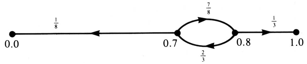
Figure 1
For n ≥ 0 with probability 1/8[(7/8)(2/3)]n, the game has 2n doubles and then B wins 4n. With probability 7/8[(7/8)(2/3)]n · 1/3, the game has 2n + 1 doubles and then A wins 2 · 4n. Thus the expected value to A is
|
∞ Σ n=0 |
7/8 · 1/3 [(7/8)(2/3)]n 2 · 4n − |
∞ Σ n=0 |
1/8 [(7/8)(2/3)]n 4n. |
However, both of these sums are infinite. A’s expectation has both infinite positive and infinite negative components and hence must be regarded as undefined. We easily generalize this case by
Theorem 2. Let B’s doubling point be L and A’s doubling point be L + M. Set R = 1 − L − M. (Assume 0 < L, M, R.) Suppose both players accept all doubles. Then the game has undefined expectation if and only if
| 3LR ≥ M. | (13) |
Proof. The situation is exactly as in the example, with terms of the form
[LR/(L + M)(R + M)]n4n.
Under assumption (13), 4LR/(L + M)(R + M) ≥ 1; hence the expectation becomes undefined.
As an example, suppose L = R = 0.35, M = 0.3. Then (13) holds and the expectation is undefined. Intriguingly, this is the doubling strategy advocated by many backgammon experts. It certainly will lead to an exciting game.
What effect does all this have on the practical player? Our answer is: “Essentially none.” There are some critical differences between the “pure” game and any real game.
Suppose that the number of doubles by each player is limited to n. Since this limits the stakes to 4n, infinite expectations cannot occur. We have shown in our paper (Keeler et al. 1969) that the appropriate first doubling point is then α(n) = 0.8 + (−1)n/5 · 4n, which rapidly approaches 0.8.
What are the practical implications of Theorem 2 if, e.g., L = R = 0.35? Since the actual game is not continuous, the expectations are finite. In the pure game the expected value of the stake (that is, the amount that changes hands) is infinite. The closer a real game may be mirrored by a continuous game, the larger the expected stake will be. If, e.g., the game consists of watching a random walk on [0, 1] with steps of 10−6, the expected stake will be large indeed, We do not see how to estimate the expected stake in backgammon itself, where—as a very practical problem—it is nearly impossible to calculate the probability of winning with any precision except in the endgame.
In the pure game, if A’s doubling point equals L + M = 0.8, there will be undefined expectations if B’s doubling point equals L ≥ 0.5. Even more subtle possibilities may occur. If B’s nth doubling point is Ln = 0.5 − εn, where εn rapidly approaches zero, then, with all doubles accepted, there will be undefined expectations. However, there are “reactive” strategies for A that avoid infinite expectations. Essentially, one accepts “absurd” doubles but does not redouble. The following strategy gives finite nonnegative expectation for A against any strategy for B.
Reactive Strategy: Initially, A’s doubling point is 0.8. If B doubles at p:
Of course, one may do better against poor players by fine-tuning the doubling point.
P.J. Orth
Santa Ana, California
(Received February 23, 1976)
From the definitions of their article, where K is the stake of the game and α the probability of winning, −K = −2Kα + 2K(1 − α) and α = 0.75. Thus, when the probability of winning first reaches 0.75, the player doubles. The value of having the sole right to double is one-third the stake of the game: 2/3 K − 1/3 K = 1/3 K.
It is interesting to note that when both players have the right to double exactly once, the first player to attain a 13/16 probability of winning should double, and the second player should redouble if his probability of winning increases to 0.75. When infinite alternate doubling is allowed, then the correct value at which to double is 0.8, as given in their article.
![]()
|
| Scan of original article from Operations Research, Vol. 23, No. 6. |
|
| "On Optimal Doubling in Backgammon," by Zadeh and Kobliska, 1977. |
|
| Articles by Emmet Keeler |
|
| Articles by Joel Spencer |
|
| Articles on cube theory |
|
Return to: Backgammon Galore |
|