|
|
Backgammon AI |
Experiences in Evaluation with BKG,
| ||||||||||||||||||||||||||||||||||
|
Originally published in Proceedings of IJCAI, 1977 (1979), pp. 428–433. This work was supported by the Advanced Research Projects Agency of the Office of the Secretary of Defense (contract F44620-73-C-0074) and is monitored by the Air Force Office of Scientific Research. |
|
Abstract. Because of very high branching factors, a backgammon program must rely on knowledge rather than search for performance. We here discuss insights gained about the structure of evaluation functions for a large domain such as backgammon. Evaluation began as a single linear polynomial of backgammon features. Later, we introduced state-classes, each with its own evaluation function. This improved the play, but caused problems with edge-effects between state-classes. Our latest effort uses models of position potential to select across the set of best members of each represented state-class. This has produced a significant jump in performance of BKG.
Because of the localization of knowledge, state-classes permit relatively easy modification of knowledge used in evaluation. They also permit the building of opponent models based upon what evidence shows the opponent knows in each state-class. Our program plays a generally competent game at an intermediate level of skill. It correctly solves a high percentage of intermediate level problems in books. |
|
Contents |
In a game such as chess, it has been customary to search very large trees of 5000 to 2 million terminal nodes. In such a paradigm, the execution of a terminal evaluation function requires a certain amount of time, which must then be multiplied by the expected number of terminal nodes in the search. Thus designers of chess programs are very circumspect in creating evaluation functions which require lengthy execution times. For this reason certain features that are not trivial to compute are usually left out, so that the program may operate faster and search more. Since there can be little or no searching in a practical backgammon program, these contingencies will not apply. On the contrary, it is desirable to apply all possible knowledge to successor positions of the root node, in an attempt to find the best next move. Further, the fact that modern backgammon involves doubling places an even greater emphasis on the use of knowledge, since it requires an understanding of a position (not just the ability to discriminate the best move) to know when to double and when to accept or refuse.
BKG now plays a completely legal game of backgammon. It is capable of doubling and accepting or refusing doubles at all times. It will also resign positions in which there is no possibility of winning, and accept resignations when there is no possibility of it winning a gammon.
We note that since there are only 15 men on a side, it is impossible to have more than 7 blockading points. For each combination of zero to seven blockading points at a distance of 1 to 12 spaces in front of a man, we computed the number of rolls that could legally be played by the blockade runner. This number was put into a table associated with the blockading pattern. This allows quick lookup of the degree to which each man is blockaded.
To support decision making during the bearing off phase, BKG has extensive tables which give the probability for a given position of one side, of bearing off all men in 1, 2, . . ., 8 rolls and the expected number of rolls (ENR) to bear all men off. The tables cover all situations for up to and including 8 men in the home board, and up to and including 25 pips worth of men in the home board.
The use of the tables in move selection is simple. BKG moves to the position with the lowest ENR. There are two exceptions to this case; that is when it is far behind or far enough ahead to have a chance of winning a gammon. In the former case, it moves to the position which has the greatest probability of bearing all men off in the number of rolls that are expected for the opponent to get off. When it is far ahead, it moves to the position which gives it the greatest chance of bearing all men off in the number of rolls it expects to have before the opponent gets his first man off.
For doubling and accepting doubles the situation is more intricate. Whenever BKG can legally double during this phase, or when it has been doubled, it executes a win probability calculation. If the positions of both sides can be looked up in the tables, then BKG can calculate the exact probability of the side on move winning by iteratively calculating the probability that the side on move will get all its men off on this roll, and then changing whose move it is, until the sum of the probabilities = 1.0. If both positions cannot be looked up, the win probability calculation is based on adjusted pipcount of both sides, but this is notably less accurate than the table lookup method, which performs superlatively.
The power of the bear-off tables is very impressive. To illustrate the type of thing BKG does to amaze its author, we show an example.
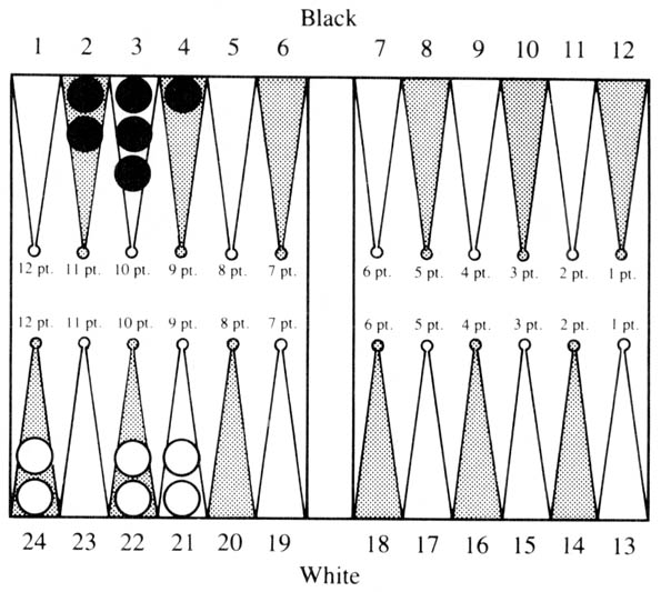
Figure 1
In the bottom part of Figure 1, White is to play a 6-2. The 6 must obviously be played from the 21 point. But what is the correct way to play the 2? Almost every human player would say 21/23. However, this is not correct; 22/24 is better. The bear-off tables report the respective ENR’s to be 2.748 and 2.739. Upon examination, it turns out that all sequences of future rolls produce the same results in the two positions except when one of the next two rolls is 1-1. If this occurred, it would leave men on the 21 and 23 points with the preferred play, which allows 6 additional combinations of getting them both off on the next roll over the other way of playing it.
The second example in the top part of Figure 1 has similar features. Here Black is to play a 6-1. The 6 must be played from the 4 point; the question is how to play the 1. Again human players would automatically play 2/1, but this is incorrect. 3/2 is correct because of future double 2’s. For these two examples it would seem that the rule: “When there are a small odd number of men on the board, play to maximize use of doubles” would seem to be the correct way for humans to capture the knowledge that is contained in the tables. This illustrates that at times precise calculation will outdo good intuition.
Therefore, we began partitioning the state-space into state-classes. The issues associated with state-classes are these: We assume that it is possible partition all states in the state-space into mutually exclusive state-classes. This is not difficult and can be accomplished by merely having recognizers for a set of state-classes, invoking these recognizers in a canonical order, and putting all non-recognized states into a grab-bag class. We further assume that within a state-class, a linear polynomial function exists which can order the members of this class according to goodness. It is apparent that this is true in the limit, when there is a state-class for each state; however, the degree to which this is possible when there are a large number of members in a given class is not clear. In practice it is possible to get very good (if not perfect) orderings, and to split a state-class when the ordering procedure becomes too complex.
This approach produced a significant improvement, but also brought some additional problems to the forefront. Whenever it was normal to progress from one state-class to another, but such a transition required the program to submit to temporary danger, it would not do so unless there was no safe alternative. With this organization as with earlier ones, BKG was unwilling to take any unforced risk, since it had no understanding of the advantages that could be accrued if the risk succeeded, but did understand the dangers of the risk. Another cause of vacillation comes up when a reshaping of the advantage is required in the transition. This can occur when the new state-class does not value highly what is valued highly in the old state-class. An example of this would be reluctance to give up containment of enemy men in order to make a transition to a superior running game position. This type of problem occurs in chess too.
To correct the above problems within the framework of the linear polynomial, it would be necessary to pinpoint where postponing the taking of the risk could no longer be justified, or when a certain advantage had outlived its usefulness.
We tried to overcome these problems by having some functions which were invoked only when a change of state-class occurred. This type of recognition produces in effect a different state-class for two identical positions, given that one is reached from a member of the same state-class and the other not. We found this to be a very difficult method of doing business that did not look anything like a long term solution to the problem.
The purpose of having state-classes was to get away from the purely linear relations among terms in the evaluation function. This way we could emphasize certain features that would have a strong impact on future situations derivable from the current state-class. Such features include the stability (likelihood of being hit in the case of backgammon) of the state, and measures of the degree of difficulty in making further progress. Usually, the side that is closest to winning will want more stable positions, and the side that is closest to losing more unstable ones. However, this is not always the case. The side that has a slightly better position may want to introduce some instability in the hope it will result in an even more favorable position (or even won), while risking losing the advantage or possibly getting slightly the worse of it. This kind of decision is very difficult to program, unless the terms in the evaluation function interact with one another. However, the edge-effect situation between state-classes became extremely difficult to overcome.
Actually, notions such as progress and risk are crutches that are not needed when a universal measure of goodness such as expectation exists, as it does in backgammon. Thus we should always move to the state with the greatest expectation, and state-classes are not needed at all. However, this is only in a system with perfect knowledge. When there is imperfect knowledge, such crutches appear necessary.
Therefore, our present system attempts to overcome edge-effects in the following way: For each applicable state-class, the best member is chosen by the linear polynomial for that state-class. Then we compute the expectation associated with each selected state-class representative, and choose the one with the highest expectation as the actual move. This has the advantage of applying the linear polynomial of a state-class to select the play with best local features, and then letting procedures with more global knowledge select the best across state-classes. The difficult part of this is to be able to compute the expectation in complicated positions. In Figure 2 below, we show how this can be done for a moderately difficult example.
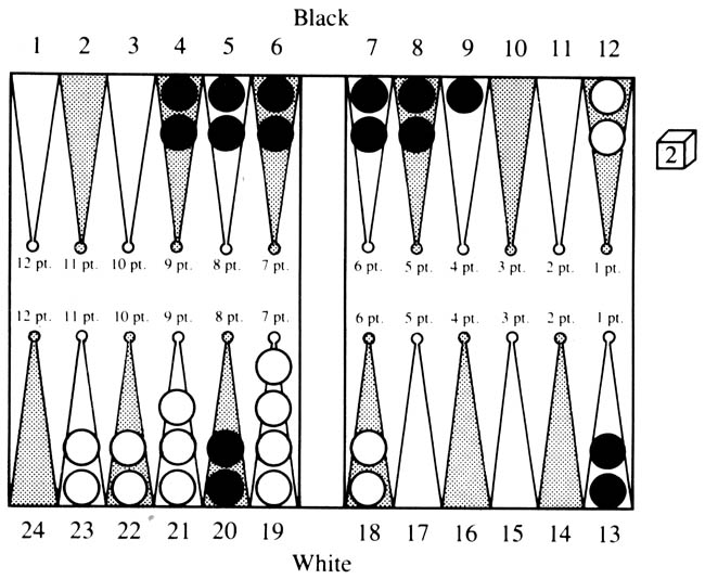
Figure 2
White is on move. The current state-class (I) is characterized by the winning side being ahead in the pipcount, having to cross exactly two more enemy points with his most-back man, and having no hittable blots. We can now imagine an evaluation function for this class which would consider the position of the doubling cube, the exact difference in the pipcount, the ease with which the most-back man can be safely moved up, the containment power of the losing side should he succeed in hitting a blot, the time lost in entering such a hit blot, and the number of pips that are available to be played as slack before any of these values are materially changed. This function would compute the expectation of White. Such a function could be derived either by analytic means or by actual simulation of positions in the class to find out how each of the above variables affected the expectation of White. Further, such a function could be tuned as experience is accumulated. Let us assume that such a function exists and predicted that in the situation of Figure 2 White should win 66% of the time, win a gammon 2% of the time, lose 30% of the time and lose a gammon 2% of the time, for a net expectation for white of +.36.
Now from this position it is possible to move to four state classes: the present one (class I), an unstable state-class where White has two points to cross, but has a blot in danger of being hit (class II), an unstable class where White has only one more point left to cross (class IV), and a stable class where White has only one point left to cross (class III). Further, if a blot is hit in state-classes II or IV, we have another state-class (V) in which White has a man on the bar which must enter in front of Black’s blocking position. For each of these state-classes an evaluation function will be able to calculate the expectation.
White’s win probability, W, in a state where he is to move is the SUM i=1 to n (Ti · Wi) where Ti is the probability of transiting to state i on the play by playing it optimally, and Wi is the probability of winning once state i is reached. If it is Black to play, White’s win probability can be computed in a like manner. This method can be used to decide between plays that result in differing state-classes even though one class may be unstable and the other not. We illustrate by an example.
Let PH denote the probability of a blot being hit on the next roll. Let Wi be the probability of winning in state-class i if the losing side is on move. Further, assume W2 = .85, W3 = .92, and W4 = .92. Then:
|
W2 = PH*W5 + (1 − PH)*W2, and W4 = PH*W5 + (1 − PH)*W4. |
To get W5 we must compute the probability of White escaping over the blockade on his next roll, as otherwise he will be doubled and will have to resign. If he does escape, he has about an even chance in the resulting position. The constants should make clear the computation below. It should be noted that when W for a side that is on roll and can double is ≥ .75 (i.e., his expectation ≥ .50) he can double and force his opponent’s resignation. Thus such terms should be ignored as their value drops to 0. This is true for instance of the term dealing with the situation where White is hit and contained.
We now use this method to decide how to play a difficult roll, 6-1, in Figure 2. There are basically two plays: run one man from the 12 point resulting in a position of class II, or play both men from the 18 point remaining in class I. For the first play:
| W |
= (1 − PH)*W2 + PH*W5 = 20/26*.85 + 16/36*2/36*.5 = .48 |
For the second play, there are 5 rolls which result in transition to state-class III (2-2, 3-3, 4-4, 5-5, 6-6), 2 rolls that result in a class II position (6-2), 8 rolls that result in class IV positions (6-1, 6-3, 6-4, 6-5), and 21 rolls that result in remaining in state-class I. The appropriate computation is: (note that W1 has dropped to .55 since White reduced his chances of bringing up his most-back man safely)
| W | = |
21*0.55/36 + 8*(16/36*2/36*0.5 + 20/36*0.85) + 5*0.92 + 2*(23/36*2/36*0.5 + 13/36*0.75) |
(I) (II) (III) (IV) |
| = | 20.61/36 = 0.57. |
Therefore, it can be seen that it is better to make play two. It should be noted that as the probability of containing a hit man varies with Black’s defensive formation, this calculation will also vary accordingly. The Wi’s we have given above are very crude and probably off by a considerable amount. However, the main purpose of this exercise was expository. As of this writing, we have implemented somewhat as sketched the state-class computations required for the above example. BKG now plays all rolls involving 6’s correctly.
The method we have described above can be used for deciding the very important problem of when to move to a state that is in a state-class different from the one we are currently in. However, the whole method assumes that an evaluation function exists for each state-class which properly orders its members, and that reasonable expectations can be produced across state-classes. At the moment we have confidence in the first part of this procedure, and the second part has been coming along extremely well.
We would still like to comment on how such a system can be improved in the face of error. For each state-class there are new state-classes that can be reached in one optimal play for each side without a capture being made. We call these classes forward with respect to the original class. Likewise, there are new classes that can be reached from the current class in one optimal play by each side, when there has been at least one capture of a man. We call these classes backward with respect to the original class.
It is possible to start with a class for which we have excellent expectation data, i.e., the class of bearing off positions that can be looked up in our tables (class B). Next, we consider all classes for which class B is forward, and improve the evaluation function for those classes, tuning the coefficients of existing terms and adding new ones as required. This will improve these evaluation functions. We also note all classes that are backward to this class, and put them on a list together with the name of the current class. We can continue this process indefinitely, but painfully until every class has been encountered. Whenever the evaluation function of a class that is on the backward list is improved, we go back and modify all the evaluation functions of the affected classes. We can then continue our process or go back to one of the classes whose function has just been modified and start anew from there. It would probably be necessary to eventually automate this procedure, if for no other reason than that eventually the evaluation functions would become so good that they would do a better job of ordering members of a class than the experimenter would. Such automation except for the introduction of new terms has been previously done by Samuel (Samuel 1959) for checkers. It would appear likely that for a game such as backgammon, it would be possible to get a selection of terms such that no new ones will ever be required. Then it will be merely a matter of tuning old evaluation functions, and occasionally trying a new (but known) term to see if it can improve prediction.
BKG has a simulation facility which can be useful in acquiring the above data. We can ask BKG to play both sides repeatedly any number of times. It will play as it ordinarily does, doubling and accepting when appropriate. BKG plays all running game positions, and those where one side is bearing off with one or fewer points to cross, nearly perfectly. Data from simulations can then be used to determine the expectation for the winning side as a function of various parameters of the original state. We have now done this for representative states of some of the simpler state-classes and used the data for fitting curves of critical variables to the statistically expected outcome. The equations derived appear reasonable, and are working out quite well in practice.
As data are collected and the evaluation functions improve, two things become possible. It is possible to keep track of how the prediction works out for the program’s own play, which can be used as an indicator of which functions need to be tuned next. It is also possible to keep track of individual opponent’s results and come to the conclusion that they don’t appraise certain state-classes correctly, and use this information in future games.
We followed the practice in scoring the results of giving BKG part credit for answers that were not perfectly correct but showed it understood the main point of the problem although the execution was not perfect. We also deducted part credit when it got the correct answer without understanding what the main problem was. Table 1 below shows the results of the tests.
Table 1. Tests of BKG on Better Backgammon.
| Position Class | Number | Right | Wrong | % Right |
|
Positional Running bearoff Engaged bearoff Back game Timing Advanced defense Defense |
28 5 11 8 13 6 3 |
18.75 5 2 3.25 4 0.5 1 |
9.25 0 9 4.75 9 5.5 2 |
67 100 22 41 31 6 33 |
| Total | 74 | 34.5 | 39.5 | 47 |
In evaluating these results, several things should be noted. The subject matter is relatively advanced, and would for the most part come up in only one of 20 or more games. There are usually on the order of three plausible answers to a problem. BKG is good enough in almost every case to know what these are; thus attaining a score of 33% or less could be regarded more or less as the result of chance. We can see that BKG is extremely good in running game play. Also it has a good understanding of the relative positional advantages. However, its performance in other intermediate level aspects of the game is at best mediocre. It has heuristics to help it do bearing off while still engaged, but these are for run-of-the-mill situations, not for the more sophisticated ones in the test set. It has no specific understanding of the back game. Since the objectives in the back game are rather different than anything else in backgammon, it will be necessary to implement a specific set of state-classes which recognize back-game potential and how to maintain and destroy it. The problem of timing is one that will be resolved soon. Essentially, this requires having a measure of how many men are presently bound to essential roles in the current evaluation, and how many pips are available to be played by the remaining men before the important men will have to be moved. BKG’s main knowledge of defense consists of its blot hitting knowledge. It does not understand the concept of coverage, i.e., controlling points on which an opponent’s blot may land in the next roll or two. It does not understand that at times it may be beneficial to expose a blot in dire circumstances or to make the “return” play. Thus this series of tests has pinpointed some specific knowledge that BKG lacks and that is not subsumed in its present knowledge base.
It is encouraging to note that even though we have just begun implementing the expectation models, BKG now gets correct 9 of the above set that it formerly got wrong.
![]()
|
| Articles by Hans Berliner |
|
| Articles on programming backgammon |
|
Return to: Backgammon Galore |
|